Decoding the Skew-T Log-P Diagram: A Complete Information to Atmospheric Thermodynamics

Associated Articles: Decoding the Skew-T Log-P Diagram: A Complete Information to Atmospheric Thermodynamics

Introduction

With enthusiasm, let’s navigate by way of the intriguing matter associated to Decoding the Skew-T Log-P Diagram: A Complete Information to Atmospheric Thermodynamics. Let’s weave fascinating data and supply recent views to the readers.

Decoding the Skew-T Log-P Diagram: A Complete Information to Atmospheric Thermodynamics

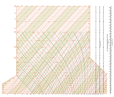
The Skew-T Log-P diagram, usually merely known as the Skew-T, is a robust device utilized in meteorology and atmospheric science to symbolize the vertical profile of atmospheric thermodynamic properties. Not like less complicated diagrams that solely present one or two parameters, the Skew-T gives a complete visualization of temperature, strain, humidity, and derived portions like dew level, stability indices, and lifted condensation ranges. This richness of knowledge makes it invaluable for understanding atmospheric processes, forecasting climate occasions, and analyzing atmospheric stability. This text will present an in depth clarification of the Skew-T Log-P diagram, its building, interpretation, and its purposes in meteorology.

Understanding the Coordinate System:

The Skew-T Log-P diagram’s identify reveals its key options:

• Skew: The temperature axis is rotated (skewed) to enhance readability and evaluation of stability. A typical skew angle is 45 levels. This rotation separates isotherms (traces of fixed temperature) and dry adiabats (traces representing adiabatic temperature modifications in dry air), making it simpler to determine atmospheric stability.

• Log-P: The strain axis is logarithmic, which means the strain intervals will not be equally spaced. This displays the exponential lower of atmospheric strain with altitude. Utilizing a logarithmic scale permits for a extra detailed illustration of the decrease environment the place most climate phenomena happen. The strain sometimes ranges from 1000 hPa (millibars) on the floor to 100 hPa (and even decrease) within the higher environment.

The diagram itself is a two-dimensional plot with strain (P) on the vertical axis and temperature (T) on the horizontal axis. Different thermodynamic parameters are overlaid as curves and features, making a complete image of the atmospheric profile.

Key Traces and Curves on the Skew-T:

A number of necessary traces and curves are plotted on the Skew-T diagram:

• Isobars (Isopleths of Stress): Horizontal traces representing fixed strain ranges. These are evenly spaced on the logarithmic scale.

• Isotherms (Isopleths of Temperature): Traces of fixed temperature. They’re slanted as a result of skew of the temperature axis.

• Dry Adiabats: Traces representing the adiabatic temperature change in a parcel of dry air because it rises or sinks. These traces slope barely to the precise. Adiabatic processes are people who happen with out warmth change with the encompassing surroundings.

• Moist Adiabats (Pseudoadiabats): Traces representing the adiabatic temperature change in a saturated parcel of air (air containing the utmost quantity of water vapor it will probably maintain at a given temperature and strain). These traces slope much less steeply than dry adiabats due to the latent warmth launched throughout condensation.

• Mixing Ratio Traces: Traces of fixed mixing ratio, representing the mass of water vapor per unit mass of dry air.

• Saturation Mixing Ratio Traces: Traces representing the utmost quantity of water vapor that may be held within the air at saturation for a given temperature and strain.

• Dew Level Traces: Traces of fixed dew level temperature. The dew level is the temperature at which the air turns into saturated and condensation begins.

• Equal Potential Temperature (θe) Traces: Traces of fixed equal potential temperature. This parameter accounts for each the smart warmth and latent warmth contained inside an air parcel. It’s a conserved amount in adiabatic, unsaturated processes.

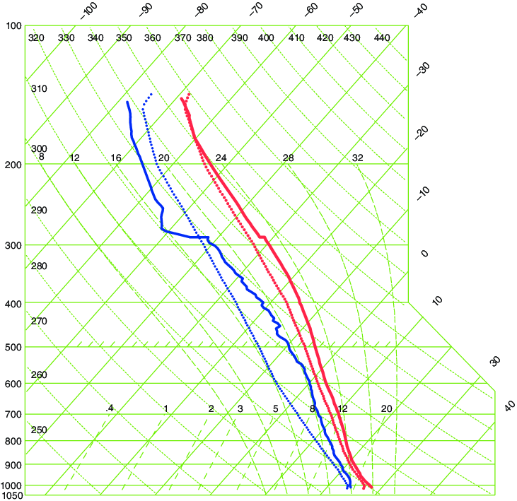
Deciphering the Skew-T:

The Skew-T gives a wealth of details about the atmospheric state:

• Temperature Profile: The temperature profile is instantly obvious from the plotted sounding (the noticed atmospheric information). Inversions (layers of accelerating temperature with peak) and isothermal layers (layers of fixed temperature) are simply recognized.

• Stability: The connection between the environmental lapse fee (the speed of temperature lower with peak within the surrounding environment) and the adiabatic lapse charges (dry and moist) determines atmospheric stability. If the environmental lapse fee is steeper than the dry adiabatic lapse fee, the environment is totally unstable. Whether it is between the dry and moist adiabatic lapse charges, it’s conditionally unstable (unstable provided that lifted above the lifting condensation stage). Whether it is shallower than the moist adiabatic lapse fee, the environment is secure.

• Lifting Condensation Degree (LCL): The LCL is the altitude at which a parcel of air, lifted adiabatically, turns into saturated and condensation begins. It’s discovered by intersecting the parcel’s temperature profile with the saturation mixing ratio line equivalent to its preliminary dew level.

• Degree of Free Convection (LFC): The LFC is the altitude at which a lifted parcel turns into hotter than its surroundings, initiating free convection.

• Equilibrium Degree (EL): The EL is the altitude at which a lifted parcel reaches impartial buoyancy (its temperature equals the environmental temperature).

• Relative Humidity: By evaluating the temperature and dew level at varied ranges, relative humidity will be estimated. Increased dew level despair (the distinction between temperature and dew level) signifies decrease relative humidity.

• Clouds: Cloud formation is indicated by the intersection of the temperature profile with the saturation mixing ratio traces. Totally different cloud sorts will be inferred based mostly on the altitude and traits of the saturation area.

Purposes of the Skew-T:

The Skew-T Log-P diagram has quite a few purposes in meteorology and atmospheric science:

• Climate Forecasting: Analyzing Skew-T soundings permits meteorologists to forecast the chance of thunderstorms, extreme climate occasions, and precipitation. Stability indices derived from the Skew-T, such because the Showalter Index, Lifted Index, and CAPE (Convective Accessible Potential Vitality), are used to evaluate convective potential.

• Aviation: Pilots and aviation meteorologists use Skew-T diagrams to evaluate atmospheric circumstances, together with icing potential, turbulence, and visibility.

• Air High quality Modeling: Understanding atmospheric stability is essential for air high quality modeling, because it influences the dispersion of pollution. Skew-T diagrams may help to foretell the transport and accumulation of pollution.

• Local weather Analysis: Skew-T diagrams can be utilized to research long-term modifications in atmospheric temperature and humidity profiles, offering insights into local weather variability and alter.

• Extreme Climate Evaluation: The Skew-T is important for understanding the dynamics of extreme thunderstorms, together with the event of supercells and tornadoes. The diagram helps determine areas of robust instability and shear, that are essential for extreme climate formation.

Limitations:

Whereas the Skew-T is a robust device, it does have some limitations:

• Spatial Decision: A single Skew-T represents the atmospheric profile at just one location. It would not seize the spatial variability of atmospheric circumstances.

• Temporal Decision: Soundings are sometimes taken at particular occasions, so the diagram solely represents the environment at that immediate. Atmospheric circumstances can change quickly.

• Mannequin Assumptions: The interpretation of the Skew-T depends on sure assumptions, similar to adiabatic processes and hydrostatic equilibrium. These assumptions might not all the time maintain true in the actual environment.

Conclusion:

The Skew-T Log-P diagram is an indispensable device for meteorologists and atmospheric scientists. Its skill to symbolize a variety of thermodynamic parameters in a visually intuitive manner makes it invaluable for understanding atmospheric processes, forecasting climate occasions, and analyzing atmospheric stability. Whereas it has limitations, its strengths far outweigh its weaknesses, solidifying its place as a cornerstone of recent meteorology. Continued developments in atmospheric modeling and information acquisition will solely improve the utility and significance of this highly effective diagramatic illustration of the environment.

Closure

Thus, we hope this text has supplied priceless insights into Decoding the Skew-T Log-P Diagram: A Complete Information to Atmospheric Thermodynamics. We admire your consideration to our article. See you in our subsequent article!